Stay up to date with all things Impira, automation, document processing, and industry best practices.
By subscribing, I agree to Botpresso’s Terms of Service and Privacy Policy.
Things You Need
Google Data Studio (Looker Studio)
Google Search Console Access
Google Sheets
Time: 10 Minutes
Step 1: Connect Google Data Studio to Google Search & Create Monthly Traffic Split
First, connect the Google Data Studio to your Google Search Console property. Create a non-brand keyword filter to eliminate factoring in the branded traffic.
In the date filter of GDS, change the date to Year Month.
Why change to Year Month? Because you are doing content decay analysis on a Month to Month basis.
Step 2: Set the preferred date range & export the table
Ideally, you should make an export of at least 3 months or 6 months to get a holistic view of the ongoing content decay.
Step 3: Import the export on Google Sheets & Prepare the Table Visualization
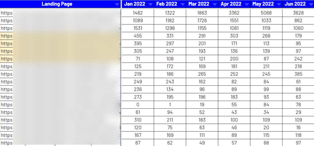
Here, you have to import the export of the table into Google Sheets. Use a helpful SUMIFS formula that will put the total clicks of the particular month for a unique URL.
The SUMIFS Formula will help you create this kind of visualization.
As you can see in the table, for every Unique URL we have got month-on-month traffic click numbers which highlight whether the number of clicks declined, progressed, or stabilized.
Without further ado, here is how to use the SUMIFS formula that will save you a ton of time.
Your GDS Export will stay in one tab where the same URL repeats often with the same months next to it. The same months would have different click numbers. The manual way would be setting filters on month & unique URL calculating the sum & paste in the unique URLs list tab.
The SUMIFS formula logic is, from GDS Export Tab you will first select the clicks column then the next selected column would be the unique URLs tab i.e. $A$2:$A,$A2, then from the GDS Export tab you will select the month column (where months repeats), then you need to mention that month as text in the Unique URL tab above you will mention that cell number in the formula.
Here is the formula you will get =SUMIFS(‘Tab1′!$C$2:$C,’Tab1′!$A$2:$A,$A2,’Tab1’!$B$2:$B,B$1)
Tab1 = GDS Export tab
Using the formula populate the SUMs on all the cells of all months. Here is the link to the Google Sheet that contains the formula & set up for you to understand it better Sheet Link
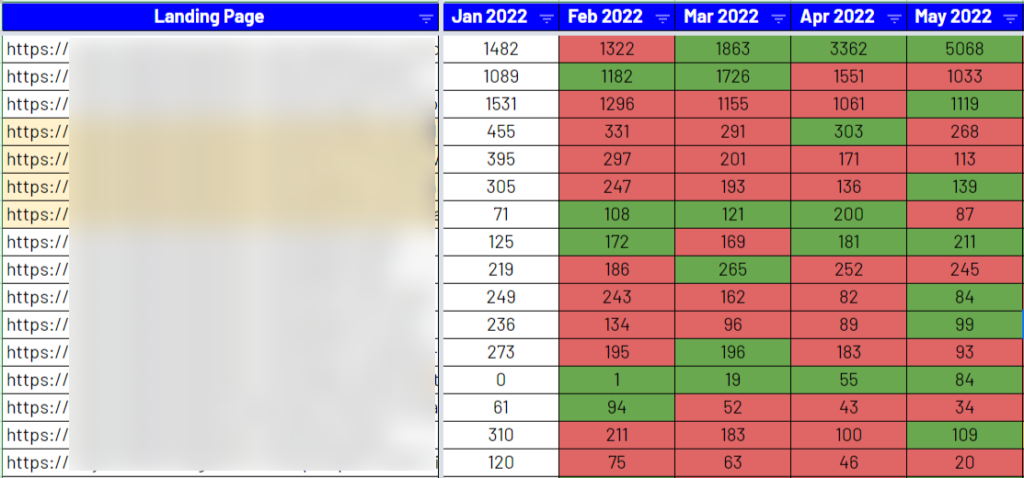
Step 4: Color Declined Clicks Tab with Conditional Formatting
This is the formula needed for the conditional formatting to work =D2>C2
You can add more conditional formatting to flag URLs that had gained with green color, and stability with yellow color.
After doing this you will get a visualization like this
Step 5: Click Drop Number from the Best Month
Add a new column next to the last month and use this formula =MAX(A2:Z2) and this formula will add the max clicks number i.e clicks of the month with max clicks.
Now you can add one more column next to & in that you can subtract the latest month clicks number with the max clicks number achieved to see if there is a drop.
This visualization will give you a birds-eye view of your content decay and at a glance. You will now understand which pages need the content optimization efforts.